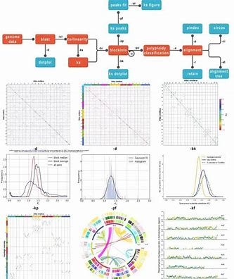
")
Polyploidy and subsequent gene loss and diploidization are present in most species and are important drivers of species evolution. If a species has undergone polyploidization during evolution, then there will be some covariant regions (i.e., the genes between two regions are paralogous homologous genes, and the order of their genes is basically the same) on the genome.
For example, Arabidopsis thaliana has undergone three ancient polyploidizations, including two diploidizations and one triploidization (Tang. et.al 2008 Science).
Of course I just remembered the conclusion before, now I’m thinking, how can I reproduce the results of this analysis?
Preparation
First of all, we need to install wgdi using conda. I usually create a new environment to avoid conflicts between the newly installed software and other software.
# Install the software
conda create -c bioconda -c conda-forge -n wgdi wgdi
# Start the environment
conda activate wgdi
After that, we download the genome, CDS, protein and GFF files from ENSEMBL
#Athaliana
wget ftp://ftp.ensemblgenomes.org/pub/plants/release-44/fasta/arabidopsis_thaliana/dna/Arabidopsis_thaliana.TAIR10.dna.toplevel.fa.gz
gunzip Arabidopsis_thaliana.TAIR10.dna.toplevel.fa.gz
wget ftp://ftp.ensemblgenomes.org/pub/plants/release-44/fasta/arabidopsis_thaliana/cds/Arabidopsis_thaliana.TAIR10.cds.all.fa.gz
gunzip Arabidopsis_thaliana.TAIR10.cds.all.fa.gz
wget ftp://ftp.ensemblgenomes.org/pub/plants/release-44/fasta/arabidopsis_thaliana/pep/Arabidopsis_thaliana.TAIR10.pep.all.fa.gz
gunzip Arabidopsis_thaliana.TAIR10.pep.all.fa.gz
wget ftp://ftp.ensemblgenomes.org/pub/plants/release-44/gff3/arabidopsis_thaliana/Arabidopsis_thaliana.TAIR10.44.gff3.gz
gunzip Arabidopsis_thaliana.TAIR10.44.gff3.gz
Note: cDNA and CDS are not the same, CDS only includes the sequence between the start codon and the stop codon, whereas cDNA will also include the UTR.
Data Preprocessing
Data preprocessing is the longest step because the software asks for input in a format other than the one you have at hand, and you usually need to do some conversion to get it in the desired form.
wgdi requires three types of information, BLAST, gene location and chromosome length, in the following formats
BLAST for the -outfmt 6 output file
Gene location information: tab-delimited chr, id, start, end, strand, order, old_id (not really in GFF format).
Chromosome length information and the number of genes on the chromosome, in the format chr, length, gene number
Also, for each gene we only need one transcript, and I usually use the longest transcript as a representative of that gene. I wrote a script (get_the_longest_transcripts.py) to extract the longest transcripts for each gene, and I wrote a new script to generate two input files for wgdi from the reference genome and the annotated GFF file at https://github.com/.xuzhougeng/myscripts/blob/master/comparative/generate_conf.py
pytho generate_conf.py -p ath Arabidopsis_thaliana.TAIR10.dna.toplevel.fa Arabidopsis_thaliana.TAIR10.44.gff3The output files are ath.gff and ath.len.
Since the ID numbering of GFF on ENSEMBL does not match that of pep.fa and cds.fa, it simply means that the numbering is preceded by a “gene:” and a “transcript:” . It is as follows
$ head ath.gff
1  gene:AT1G01010  3631  5899  +  1  transcript:AT1G01010.1
1  gene:AT1G01020  6788  9130  -  2  transcript:AT1G01020.1
1  gene:AT1G01030  11649  13714  -  3  transcript:AT1G01030.1
1  gene:AT1G01040  23416  31120  +  4  transcript:AT1G01040.2
1  gene:AT1G01050  31170  33171  -  5  transcript:AT1G01050.1
1  gene:AT1G01060  33379  37757  -  6  transcript:AT1G01060.3
1  gene:AT1G01070  38444  41017  -  7  transcript:AT1G01070.1
1  gene:AT1G01080  45296  47019  -  8  transcript:AT1G01080.2
1  gene:AT1G01090  47234  49304  -  9  transcript:AT1G01090.1
1  gene:AT1G01100  49909  51210  -  10  transcript:AT1G01100.2
So I used sed to remove the information.
sed -i -e 's/gene://' -e 's/transcript://' ath.gffIn addition, pep.fa, cds.fa contain all the genes with long names, and we don’t need the “.1”, “.2” part of the genes.
$ head -n 5 Arabidopsis_thaliana.TAIR10.cds.all.fa
>AT3G05780.1 cds chromosome:TAIR10:3:1714941:1719608:-1 gene:AT3G05780 gene_biotype:protein_coding transcript_biotype:protein_coding gene_symbol:LON3 description:Lon protease homolog 3, mitochondrial [Source:UniProtKB/Swiss-Prot;Acc:Q9M9L8]
ATGATGCCTAAACGGTTTAACACGAGTGGCTTTGACACGACTCTTCGTCTACCTTCGTAC
TACGGTTTCTTGCATCTTACACAAAGCTTAACCCTAAATTCCCGCGTTTTCTACGGTGCC
CGCCATGTGACTCCTCCGGCTATTCGGATCGGATCCAATCCGGTTCAGAGTCTACTACTC
TTCAGGGCACCGACTCAGCTTACCGGATGGAACCGGAGTTCTCGCGATTTATTGGGTCGTb
With the help of seqkit, I filtered and renamed the original data.
seqkit grep -f <(cut -f 7 ath.gff ) Arabidopsis_thaliana.TAIR10.cds.all.fa | seqkit seq --id-regexp "^(.*?)\\.\\d" -i > ath.cds.fa
seqkit grep -f <(cut -f 7 ath.gff ) Arabidopsis_thaliana.TAIR10.pep.all.fa | seqkit seq --id-regexp "^(.*?)\\.\\d" -i > ath.pep.fa
Protein intercomparison was performed by NCBI BLASTP or DIAMOND with output format -outfmt 6
makeblastdb -in ath.pep.fa -dbtype prot
blastp -num_threads 50 -db ath.pep.fa -query ath.pep.fa -outfmt 6 -evalue 1e-5 -num_alignments 20  -out ath.blastp.txt &
Covariance analysis
Plotting a Bitmap
At the end of the above steps, it is actually very simple to plot the dot plot, just create the configuration file, then modify the configuration file, and finally run wgdi.
The first step is to create a configuration file
wgdi -d \? > ath.confThe information in the configuration file is as follows (the information below is just to explain the parameters and does not need to be copied)
[dotplot]
blast = blast file
gff1 = gff1 file
gff2 = gff2 file
lens1 = lens1 file
lens2 = lens2 file
genome1_name = Genome1 name
genome2_name = Genome2 name
multiple = 1 # number of best homologs, indicated by red dots in the blast output
score = 100 # Score filtered by blast output
evalue = 1e-5 # evalue filter for blast output
repeat_number = 20 # Maximum number of homologs in genome2 relative to genome1.
position = order
blast_reverse = false
ancestor_left = none
ancestor_top = none
markersize = 0.5 # dot size
figsize = 10,10 # image size
savefig = savefile(.png,.pdf)
The second step is to modify the configuration file. Since this is a self-comparison, the contents of gff1 and gff2 are the same, and the contents of lens1 and lens2 are the same.
[dotplot]
blast = ath.blastp.txt
gff1 =  ath.gff
gff2 =  ath.gff
lens1 = ath.len
lens2 = ath.len
genome1_name =  A. thaliana
genome2_name =  A. thaliana
multiple  = 1
score = 100
evalue = 1e-5
repeat_number = 5
position = order
blast_reverse = false
ancestor_left = none
ancestor_top = none
markersize = 0.5
figsize = 10,10
savefig = ath.dot.png
Finally, run the following command
wgdi -d ath.conf
Dot Matrix Diagram
From the figure, we can easily observe three colors, which are red, blue, and gray. In WGDI, the red color indicates the optimal homologous (highest similarity) match of genome2’s genes in genome1, the next best four genes are blue, and the remaining part is for gray. The segments appearing diagonally in the figure are not self matches, as WGDI has filtered out the self over self results. The question then arises, what are these genes? This question will be answered in a subsequent analysis.
If there is a doubling event in the genome, then for one region of the genome there may be another region with genes that are similar to it (homologous genes) and these genes are arranged in a more consistent order. This is reflected in a dot plot, where a “line” of dots can be observed. The lines need to be in quotation marks because when you zoom in, you will see that they are still dots.

Enlargement of some regions
Since the further identification of the covariate region is based on these “points”, the parameters affecting whether these points are homologous or not are very important, i.e. score,evaluate,repeat_number in the configuration file.
Covariance analysis and Ks calculation
For synteny and collinearity, it is generally believed that synteny refers to a certain number of homologous genes in two regions, and there is no requirement for gene order placement. Collinearity is a special form of homozygosity that requires a similar ordering of homologous genes.
The -icl module (Improved version of ColinearScan) has been developed by wgdi for covariance analysis, which is very simple to use, and it also creates a configuration file first.
wgdi -icl \? >> ath.confThen make changes to the configuration file.
[collinearity]
gff1 = ath.gff
gff2 = ath.gff
lens1 = ath.len
lens2 = ath.len
blast = ath.blastp.txt
blast_reverse = false
multiple  = 1
process = 8
evalue = 1e-5
score = 100
grading = 50,40,25
mg = 40,40
pvalue = 0.2
repeat_number = 10
positon = order
savefile = ath.collinearity.txt
The evalue, score is related to the filtering of BLAST files for homologous gene pairs. multiple determines the best compared genes, repeat_number indicates the maximum number of genes allowed to be potential homologous genes, grading scores homologous genes based on how well they match, and mg refers to the maximum number of vacancies allowed in the covariance region. genes in the covariate region.
After running the results, you will get ath.collinearity.txt to record the covariance region. Lines starting with # record meta-information about the covariance region, such as score, pvalue, number of pairs of genes (N) etc.
grep '^#' ath.collinearity.txt | tail -n 1
# Alignment 959: score=778.0 pvalue=0.0003 N=16 Pt&Pt minus
Immediately after that, we can compute Ks based on the covariance results.
The same is also done by first generating the configuration file
wgdi -ks \? >> ath.confThen modify the configuration file. We need to provide cds and pep files, covariance analysis output file (support covariance analysis results from MCScanX).WGDI will use muscle to associate based on protein sequences, then use pal2pal.pl to convert protein associations to codon associations based on cds sequences, and finally calculate ka and ks using yn00 in paml.
[ks]
cds_file =   ath.cds.fa
pep_file =   ath.pep.fa
align_software = muscle
pairs_file = ath.collinearity.txt
ks_file = ath.ks
The ks calculation takes a while, so it may be worthwhile to understand Ka and Ks when doing so.Ka and Ks refer to the number of non-synonymous substitution sites, and the number of synonymous substitution sites, respectively. According to the neutral evolution hypothesis, most of the changes in genes are neutral mutations that do not affect the survival of the organism, so when a pair of homologous genes are separated earlier, the number of base substitutions that do not affect the survival is higher (Ks), and vice versa.
After running the results, the output Ks file has 6 columns corresponding to the Ka and Ks values for each gene pair.
$ head ath.ks
id1  id2  ka_NG86  ks_NG86  ka_YN00  ks_YN00
AT1G72300  AT1G17240  0.1404  0.629  0.1467  0.5718
AT1G72330  AT1G17290  0.0803  0.5442  0.079  0.6386
AT1G72350  AT1G17310  0.3709  0.9228  0.3745  1.071
AT1G72410  AT1G17360  0.2636  0.875  0.2634  1.1732
AT1G72450  AT1G17380  0.2828  1.1068  0.2857  1.5231
AT1G72490  AT1G17400  0.255  1.2113  0.2597  2.0862
AT1G72520  AT1G17420  0.1006  0.9734  0.1025  1.0599
AT1G72620  AT1G17430  0.1284  0.7328  0.1375  0.603
AT1G72630  AT1G17455  0.0643  0.7608  0.0613  1.2295
Given that the covariance and Ks value outputs are too informative to be convenient to use, a better approach would be to aggregate the two to get summarized information about the individual covariance regions.
WGDI provides the -bi parameter to help us with data integration. The same goes for generating the configuration file
wgdi -bi ? >> ath.confModify the configuration file. Collinearity and ks are the output files from the first two steps, and ks_col declares which column from the ks file to use.
[blockinfo]
blast = ath.blastp.txt
gff1 =  ath.gff
gff2 =  ath.gff
lens1 = ath.len
lens2 = ath.len
collinearity = ath.collinearity.txt
score = 100
evalue = 1e-5
repeat_number = 20
position = order
ks = ath.ks
ks_col = ks_NG86
savefile = ath_block_information.csv
Just run it.
wgdi -bi ath.confThe output file is stored in csv format, so it can be opened directly in EXCEL, with 11 columns.
- id is the unique identifier of the covariate result.
- chr1,start1,end1 is the covariance range of the reference genome (left side of the dot plot).
- chr2,start2,end2 i.e. the covariance range of the reference genome (the upper side of the dot plot).
- pvalue is the evaluation of the covariance result, and it is often considered to be more reasonable if it is less than 0.01.
- length is the length of the covariate segment
- ks_median i.e. the median of all gene pairs of ks in the covariate (mainly used to judge the distribution of ks)
- ks_average i.e. the average value of all gene pairs of ks in the covariate.
- homo1,homo2,homo3,homo4,homo5 are related to the multiple parameter, i.e. there are a total of homo+multiple columns.
The main rule is that gene pairs are assigned a value of 1 if they are red in the dot plot, 0 if they are blue, and -1 if they are grey (for colors, refer to the previous tweet about wgdi dot plots). All pairs of genes on the covariate segment are assigned values and then averaged, thus giving the covariate a value of -1,1. If the points of the covariate are mostly red, then the value is close to 1. This can be used as a filter for covariate segments.
- block1,block2 are the positions of the gene order on the covariate fragment, respectively.
- The ks value of the upper gene pair of the covariate fragment.
- density1,density2 The density of the gene distribution of the covariate fragment. Smaller values indicate sparseness
This table is a focus for subsequent exploratory analysis, for example, we can use it to analyze the genes that appear on the diagonal in our dot plot. The code below is extracting all the genes in the first covariate region, and then performing enrichment analysis to plot a bubble map.
df <- read.csv("ath_block_information.csv")

tandem_length <- 200

df$start <- df$start2 - df$start1
df$end <- df$end2 - df$end1

df_tandem <- df[abs(df$start) <= tandem_length |
     abs(df$end) <= tandem_length,]

gff <- read.table("ath.gff")

syn_block1 <-  df_tandem[1,c("block1", "block2")]

gene_order <- unlist(
  lapply(syn_block1, strsplit, split="_", fixed=TRUE, useBytes=TRUE)
)

gene_order <- unique(as.numeric(gene_order))


syn_block1_gene <- gff[ gff$V6 %in% gene_order, "V2"]

#BiocManager::install("org.At.tair.db")
library(org.At.tair.db)
library(clusterProfiler)

ego <- enrichGO(syn_block1_gene,
                OrgDb = org.At.tair.db,
                keyType = "TAIR",ont = "BP"
                )
dotplot(ego)
Bubble diagram
Further observation of these genes reveals that the genes are numbered back-to-back, suggesting that this cluster of genes has something to do with pollen recognition.
> as.data.frame(ego)[1,]
                   ID           Description GeneRatio  BgRatio       pvalue
GO:0048544 GO:0048544 recognition of pollen    11/560 43/21845 7.794138e-09
               p.adjust      qvalue
GO:0048544 8.121073e-06 7.95418e-06
                                                                                                                  geneID
GO:0048544 AT1G61360/AT1G61370/AT1G61380/AT1G61390/AT1G61400/AT1G61420/AT1G61440/AT1G61480/AT1G61490/AT1G61500/AT1G61550
           Count
GO:0048544    11